Review
The CAPM suggests that a firm’s expected excess return (Ri) above the risk-free rate (Rf) is simply a scaled version of the market portfolio (Rm) expected excess return. Risk-free rate can be the rate of return on US treasury bonds. In other words: ( Ri - Rf ) = scaling factor * ( Rm - Rf ). Put differently,
( Ri - Rf ) = alpha + beta * ( Rm - Rf ).
Gene Fama and Ken French argued convincingly that there are additional risk factors that can better describe the expected excess return, namely a size premium (SMB) and a value premium (HML). Recent research has shown that the expected return can further be improved with additional factors beyond size and value. Cliff Asness eloquently describes them as follows:
-
Premium Factors
-
RM-RF - The return spread between the capitalization weighted stock market and cash.
-
SMB - The return spread of small minus large stocks (i.e., the size effect).
-
HML - The return spread of cheap minus expensive stocks (i.e., the value effect).
-
RMW - The return spread of the most profitable firms minus the least profitable.
-
CMA - The return spread of firms that invest conservatively minus aggressively.
-
With this knowledge, how can you evaluate the exposure a portfolio has to these risk factors?
Regression
By re-expressing the CAPM to use the additional risk factors, the regression can be expressed as:
( Ri - Rf ) = alpha + beta1 * ( Rm - Rf ) + beta2 * HML + beta3 * SMB + beta4 * RWM + beta5 * CMA
Ken French maintains a library of factors for doing exactly these kinds of regressions. You can access it here.
One of the most famous portfolio managers of the 20th century is Peter Lynch, who was the PM for Fidelity’s Magellan Fund. What were his factor exposures during the time he was managing the fund, from 1977 to 1990?
The regression results follow:
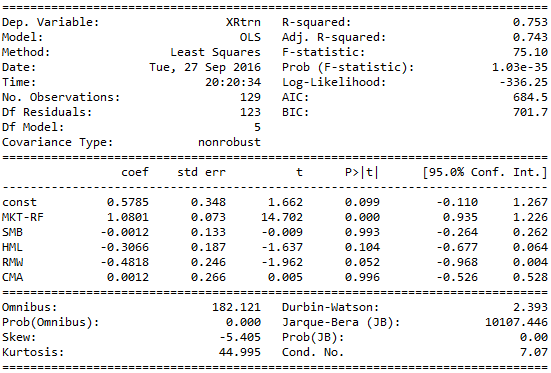
Obviously, his fund had a statistically strong positive relationship with the market (MKT-RF), and clearly a statistically strong negative relationship with HML and RMW factors. The negative relationship with HML suggests he was exposed to more growth stocks than value stocks, and firms that were least profitable rather than most profitable. Given the small t-statistics to SMB and CMA we can not make statistically significant conclusions as to his portfolio’s exposures to these risk factors.
Remember when you are running such regressions, subtract out the risk free rate from the returns of the market and the security or fund you are analyzing. While the current ZIRP regime we’re currently in won’t make much of a difference, when you go back to the 80s and 90s it definitely will.
How to hedge?
The analysis above, the risk factors are not tradable. Within the past few years, however, there has been a large increase in the number of exchange traded funds that provide factor exposure. If you, as an investor in the Magellan fund, wanted to hedge the exposure to growth stocks (HML factor), you can simply buy $0.30 worth of a fund that tracks HML for each $1.00 that is invested in Magellan:
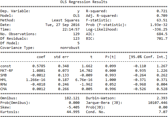
After running the same regression, you can now see that the coefficient and t-statistic for the HML factor are effectively zero. In practice, use an ETF that is both easily shortable with low short-rate fee to achieve the best results.
Python Code
This code is adapted from the solid work by nakulnayyar. It has been changed to use the new five factor model, and show an example of hedging.
import pandas as pd
import numpy as np
from StringIO import StringIO
from zipfile import ZipFile
from urllib import urlopen
import pandas.io.data as web
import statsmodels.api as sm
url = urlopen("http://mba.tuck.dartmouth.edu/pages/faculty/ken.french/ftp/F-F_Research_Data_5_Factors_2x3_CSV.zip")
zipfile = ZipFile(StringIO(url.read()))
FFdata = pd.read_csv(zipfile.open('F-F_Research_Data_5_Factors_2x3.CSV'),
                     header = 0, names = ['Date','MKT-RF','SMB','HML','RMW','CMA','RF'],
                     skiprows=3)

FFdata = FFdata[:638]

//#Convert YYYYMM into Date
FFdata['Date'] = pd.to_datetime(FFdata['Date'], format = "%Y%m")
FFdata.index = FFdata['Date']
FFdata.drop(FFdata.columns[0], axis=1,inplace=True)

#Drop Days in YYYY-MM-DD
FFdata.index = FFdata.index.map(lambda x: x.strftime('%Y-%m'))

#Convert into float
FFdata = FFdata.astype('float')
FFdata.tail()

#Get Data from Yahoo
start = datetime(1980,1,1)
end = datetime(1990,10,1)
f = web.get_data_yahoo("FMAGX", start, end, interval='m')

#Delete Columns
f.drop(f.columns[[0,1,2,3,4]], axis=1, inplace=True)
#Fix Date Column
f.index = f.index.map(lambda x: x.strftime('%Y-%m'))

f['Return'] = f['Adj Close'].pct_change().shift(0) * 100.0
f.head()


data2 = pd.concat([f,FFdata], axis = 1)
data2['XRtrn'] = (data2['Return'] - data2['RF'])
df = data2[np.isfinite(data2['XRtrn'])]
df.tail()


y = df['XRtrn']


X = df.ix[:,[2,3,4,5,6]]
X = sm.add_constant(X)
model = sm.OLS(y, X)
results = model.fit()
print(results.summary())

y.plot()

#Hedge HML
y1 = y - results.params[3] * df['HML']

model = sm.OLS(y1, X)
results = model.fit()
print(results.summary())